A step-by-step guide to object recognition using Python

I recently got into Python object recognition and this is a guide detailing steps to build your own model.

Author

Affiliation

Sid Metcalfe

Cartesian Mathematics Foundation

Published

November 22, 2023

Introduction

I’ve always been intrigued by how our brains can effortlessly identify objects, a task that’s notoriously complex for machines. Dabbling in Python, I discovered a universe of libraries designed to mimic this very human skill of object recognition. As a beginner, I was amazed by how a few lines of code could empower computers to ‘see’. In this article, I’ll walk you through the exhilarating process of teaching a machine to recognize objects, from setting up your Python environment to evaluating your model’s performance. It’s a journey filled with learning curves, but the reward of watching your creation correctly identify an object is immeasurably delightful.

Introduction to Object Recognition and Python Libraries

Object recognition is a fascinating facet of machine learning, where machines learn to identify and classify objects within images. It’s akin to teaching a child to point out apples or cats in a picture book. The realm of Python libraries for this purpose is diverse and robust, often abstracting complex algorithms into simple-to-use functions.

Before diving into libraries, you must grasp the basic idea: object recognition involves feeding an image into an algorithm that processes and identifies the objects within it. For a practical guide on implementing this with Python, you can refer to Person detection in video streams using Python in 2023: a tutorial. It’s a remarkable blend of computer vision and machine learning techniques, ensuring the machine ‘sees’ and ‘understands.’

Now, let’s begin our journey by exploring some Python libraries that make it feasible for beginners like myself to get started without getting lost in the mathematical abyss.

from skimage import io

# Load an image from the web
image_url = 'http://example.com/path/to/image.jpg'
image = io.imread(image_url)

scikit-image is one of the libraries I first used. This code snippet flawlessly fetches an image from a URL. Simple, isn’t it? But object recognition requires more than just image retrieval.

from PIL import Image

# Load an image from a file
image_path = '/path/to/local/image.jpg'
image = Image.open(image_path)

PIL or Pillow, a fork of PIL, is another staple for image handling. It’s a perfect tool for the initial steps of image processing, like opening or saving images in varying formats.

However, when it’s time to truly dive into object recognition, you’ll likely encounter OpenCV (Open Source Computer Vision Library). With a plethora of functions targeting real-time computer vision, it’s a powerhouse for enthusiasts.

import cv2

# Convert the image to grayscale
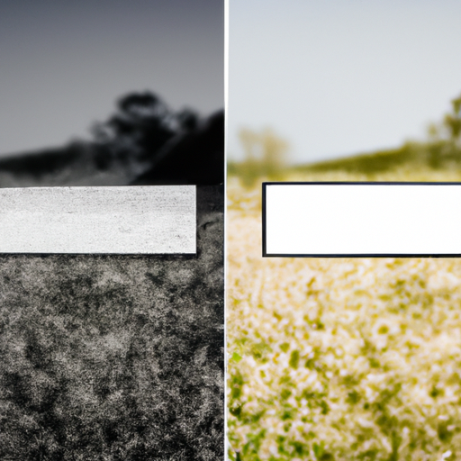
gray_image = cv2.cvtColor(image, cv2.COLOR_BGR2GRAY)

Grayscale conversion is a common preprocessing step. Why? It simplifies the image, reducing the computational load and focusing on structural features.

But we want to do more than convert images to black and white. Take TensorFlow and Keras, for instance. These libraries allow us to build and train neural networks that perform object recognition with relative ease, abstracting much of the complexity.

from keras.models import Sequential
from keras.layers import Dense

# A simple Neural Network model for illustration
model = Sequential([
    Dense(32, activation='relu', input_shape=(784,)),
    Dense(10, activation='softmax'),
])

Here, I’ve set up a rudimentary neural network using Keras with an input layer and an output layer. This is, of course, overly simplified for complex object recognition, but it illustrates the ease of constructing neural networks.

While we can’t cover the entire process of implementing a recognition model here, the Python ecosystem makes it accessible. Libraries like TensorFlow and datasets available for practice, such as CIFAR-10, truss your learning bridge, offering a hands-on, code-first approach to understanding the magic behind object recognition.

And, as a beginner, to go beyond mere theory and witness your machine discerning cats from dogs or apples from oranges with a few lines of code is nothing short of magical. Stay tuned as we delve deeper into the nuances of object recognition models and how to yield their powers using Python.

Setting Up Your Python Environment for Image Processing

A screenshot of a python code editor with library installation commands

Setting up a proper Python environment is crucial for diving into the world of image processing. My journey began by selecting the right tools and packages to make object recognition tasks less daunting and more efficient.

First, let’s ensure Python is installed on your system. I prefer using Anaconda, a widely-used Python distribution for scientific computing that comes with a convenient package manager called conda. You can download it from the Anaconda website. Once installed, I create a new environment specifically for image processing to keep my workspace organized and dependencies in check.

conda create --name imageproc python=3.8
conda activate imageproc

Now, with our environment activated, we’re ready to install the key libraries for image processing: numpy, scipy, and, of course, opencv. NumPy is essential for handling arrays and matrices, which are inherently part of image data. SciPy provides additional functionality, like multi-dimensional image processing. OpenCV (Open Source Computer Vision Library) is the powerhouse for image processing tasks.

conda install numpy scipy
conda install -c conda-forge opencv

For more advanced image processing and object recognition features, we’ll need scikit-image and pillow. Scikit-image extends SciPy’s image processing capabilities, and Pillow is a more user-friendly fork of PIL, the Python Imaging Library.

conda install scikit-image pillow

Next, I like to add matplotlib for plotting images and visualizations - a crucial part of understanding what’s happening with the data.

conda install matplotlib

Once these are set up, your Python environment is pretty much ready to tackle some basic image processing tasks! But for object recognition, we need to go a step further and introduce machine learning into the mix. Enter scikit-learn and tensorflow (or keras, which now comes integrated with TensorFlow).

conda install scikit-learn
conda install tensorflow

With tensorflow, you gain access to a multitude of pre-trained models and tools for crafting your own models for object recognition tasks. I found starting with pre-trained models very useful to get a feel for their capabilities before diving into custom model training.

To check if everything is working correctly, I usually run a simple OpenCV code to load and display an image:

import cv2
import matplotlib.pyplot as plt

# Load an image using OpenCV
image = cv2.imread('sample.jpg')

# Convert the image from BGR to RGB (OpenCV uses BGR by default)
image_rgb = cv2.cvtColor(image, cv2.COLOR_BGR2RGB)

# Display the image using matplotlib
plt.imshow(image_rgb)
plt.show()

If a vibrant image pops up on your screen, congratulations, you’ve successfully set up your Python environment for image processing!

Setting up a tailored environment might seem tedious at first, but trust me, investing time to get the foundations right pays off immensely when you dive deeper. With a robust setup, you can iterate faster and focus on the real challenges in object recognition—understanding the models and improving performance—without being sidetracked by avoidable technical hiccups.

Loading and Preprocessing Images for Recognition

An image showing a raw photo on one side and a preprocessed version on the other

Before digging into the nitty-gritty of object recognition, it’s vital to understand how to prep images for such a task effectively. The quality of image preprocessing can make or break the model’s ability to recognize objects accurately.

I’ll kick things off by diving straight into loading images. Python and its libraries have made this task relatively straightforward. Firstly, make sure you have libraries like PIL (Pillow) or opencv-python installed.

from PIL import Image
image = Image.open('path/to/your/image.jpg')

Or, if you’re in the OpenCV camp:

import cv2
image = cv2.imread('path/to/your/image.jpg')

Once loaded, it’s not uncommon to encounter images of various shapes and sizes, while many models expect a fixed size. therefore, resizing is often essential:

from PIL import Image

image = Image.open('path/to/your/image.jpg')
image = image.resize((224, 224))  # Resize to the input size expected by the model

Or using OpenCV:

import cv2

image = cv2.imread('path/to/your/image.jpg')
image = cv2.resize(image, (224, 224))  # Resize to the input size expected by the model

Color channels can also pose an issue, with some models requiring a specific ordering (RGB vs. BGR). In OpenCV, images are loaded in BGR format by default, while many models expect RGB:

image = cv2.cvtColor(image, cv2.COLOR_BGR2RGB)  # Convert from BGR to RGB

When the image is properly sized and colored, normalization is often the next step. It involves scaling pixel values to a range that the model expects, often [0, 1] or [-1, 1]:

import numpy as np

image = np.array(image) / 255.0  # Normalize to [0, 1]

For some models, you may need to standardize the images further by subtracting the mean and dividing by the standard deviation of pixel values:

mean = np.array([0.485, 0.456, 0.406])  # Usually precomputed from a large set of images
std = np.array([0.229, 0.224, 0.225])

image = (image - mean) / std  # Standardize the image

Batch processing is a fundamental part of object recognition. It involves feeding the model multiple images at once for efficiency. To simulate this, even with a single image, we need to add an extra dimension to our data to represent the batch size:

image = np.expand_dims(image, axis=0)  # Add batch dimension

At this stage, I usually ensure my image is in the exact format the model expects. As every model is different, it’s a good practice to scour the documentation to avoid slip-ups here.

Finally, batched and preprocess the image is ready to be fed to a model for recognition. It’s worth mentioning that all these preprocessing steps can be packaged into a single function or a preprocessing pipeline, especially when dealing with large datasets.

Remember, the effectiveness of preprocessing directly impacts model performance, so it’s worth spending time to get it right. Also, keep in mind that tools and libraries evolve, so keep an eye on the latest updates to libraries like Pillow, OpenCV, and even TensorFlow and PyTorch, as they often add new utilities to streamline these tasks.

While I’ve steered clear from diving deep into model-specific preprocessing, a lot of state-of-the-art models, like those from tensorflow.keras.applications, come with their own preprocess_input function, which I highly recommend checking out for tailored preprocessing.

Choosing and Understanding Object Recognition Models

A diagram explaining the architecture of a typical object recognition model

When I first dived into the realm of object recognition models, I was immediately struck by the sheer diversity of available options. Each model, with its peculiar architecture and capabilities, shines in different scenarios. In this journey, I’ll help you navigate the landscape to select and understand an object recognition model that best suits your project’s needs.

Let’s begin by choosing a model. If you’re just starting out, a pretrained model like MobileNet or ResNet, fine-tuned on a large dataset like ImageNet, often serves as a robust foundation for many applications. Models like these strike a balance between speed and accuracy and are widely supported by many libraries. For instance, TensorFlow’s Keras API provides easy access to these models:

from tensorflow.keras.applications import MobileNetV2

# Load the MobileNetV2 model pre-trained on ImageNet data
model = MobileNetV2(weights='imagenet')

However, if you’re dealing with real-time applications where speed is critical, look towards lightweight models such as SqueezeNet or MobileNetV2, as their architecture is specifically designed for such environments:

from tensorflow.keras.applications import MobileNetV2

# Load MobileNetV2 with a specific input shape
model = MobileNetV2(input_shape=(128, 128, 3), weights=None, classes=1000)

Conversely, if accuracy is your endgame and computational resources are not a limiting factor, dive into heavier models like Inception and ResNet-50. They drill down to capture minute details, giving you state-of-the-art accuracy for image recognition tasks:

from tensorflow.keras.applications import ResNet50

# Load the ResNet50 model pre-trained on ImageNet data
model = ResNet50(weights='imagenet')

After choosing your chariot—excuse me, I mean your model—it’s time to coax a deeper understanding from it. Let’s decode the secret workings of these models by visualizing the convolutional layers, which are the workhorses of feature extraction. To obtain a glimpse of what features our model is focusing on, you can access intermediate layers of the model and feed an input image through them:

from tensorflow.keras import models
import numpy as np
import matplotlib.pyplot as plt

# Get intermediate layers from the model
layer_outputs = [layer.output for layer in model.layers[1:8]]
activation_model = models.Model(inputs=model.input, outputs=layer_outputs)

# Assuming 'img_tensor' is your preprocessed image ready for prediction
activations = activation_model.predict(img_tensor)

# Now, let's plot the features of the first conv layer
first_layer_activation = activations[0]
plt.matshow(first_layer_activation[0, :, :, 4], cmap='viridis')
plt.show()

Each convolution layer can be thought of as a lens focusing on different aspects of spatial hierarchy in an image - early layers catch basic patterns like edges and textures, while later layers amalgamate these into more complex features like ‘eyes’ or ‘wheels’.

Remember though, choosing a model is only the beginning. What follows is an exploration into hyperparameter tuning, layer customization, and feeding in the right concoction of data for the model to digest. None of this happens in a vacuum - it’s all about experimenting to see what tweaks elicit the best performance from your chosen Sibyl of image recognition.

To get the full story on a particular model’s prowess and temperament, considering scrolling through the model’s original paper or GitHub repository is a splendid idea. It’s here that you’ll find the minutiae of architectural decisions and oftentimes, pre-trained models ready for use. For example, you can read about some practical applications of machine learning models in my tutorial on Using PyTorch for image classification in 2023.

As final food for thought, always consider your model in the context of your dataset and task. Object recognition isn’t just about the particular algorithm—it’s about the union of model, data, and task. As you progress, lean on communities like those on GitHub, Stack Overflow, and Reddit’s r/MachineLearning. Their collective wisdom can guide you through the often-tangled forest of machine learning and object recognition.

Happy coding!

Implementing an Object Recognition Model with Python

A code snippet showing a python function running an object recognition model

Let’s dive in and actually build an object recognition model using Python. By this stage, you should have a good grasp of Python, its relevant image processing libraries, and a rough idea of how object recognition models work. But reading about concepts and implementing them are entirely different beasts. So, I’ll walk you through how I tackled the challenge.

First off, we need a model. There are several pre-trained models available, but for simplicity and efficiency, I chose the MobileNetV2 model through TensorFlow’s Keras API. Why? MobileNetV2 is lightweight and designed for mobile devices, making it a great candidate for our initial trials.

import tensorflow as tf

# Load the MobileNetV2 model. Exclude the top layer as we'll add our own
model = tf.keras.applications.MobileNetV2(weights='imagenet', include_top=False)

# Adding a new classifier layer for transfer learning
x = model.output
x = tf.keras.layers.GlobalAveragePooling2D()(x)
x = tf.keras.layers.Dense(1024, activation='relu')(x)
predictions = tf.keras.layers.Dense(1, activation='sigmoid')(x)

# This is the model we will train
model = tf.keras.Model(inputs=model.input, outputs=predictions)

This snippet uses the MobileNetV2 model as a base and adds a few layers at the end. I’ve opted for a simple structure with a global average pooling layer followed by a dense layer. Typically, the last layer’s activation function and number of neurons would match the problem at hand (binary, multi-class, etc.).

Once the model is set, let’s compile it. The choice of the optimizer and loss function again depends on the task’s specifics. For a binary classification, which is common in object recognition tasks where you determine whether the object is present or not, ‘binary_crossentropy’ works well.

model.compile(optimizer=tf.keras.optimizers.Adam(),
              loss='binary_crossentropy',
              metrics=['accuracy'])

Training a model can take ages, but TensorFlow fortunately allows us to utilize an ImageDataGenerator for augmenting our data and speeding up the process.

from tensorflow.keras.preprocessing.image import ImageDataGenerator

train_datagen = ImageDataGenerator(
    rescale=1./255,
    shear_range=0.2,
    zoom_range=0.2,
    horizontal_flip=True)

# Assume train_dir specifies the directory where the training data is
train_generator = train_datagen.flow_from_directory(
    train_dir,
    target_size=(224, 224),
    batch_size=32,
    class_mode='binary')

Here, I’ve set up an ImageDataGenerator to automatically apply data augmentation techniques like shearing, zooming, and flipping, which help the model generalize better from the available training data.

Training the model is straightforward with the fit function. Given the potentially large dataset and model size, I’d usually run this on a machine with decent computational power.

history = model.fit(
    train_generator,
    steps_per_epoch=1000,
    epochs=10)

Remember to track the model’s performance over epochs to ensure its learning. A common pitfall I’ve faced is overfitting, where your model learns your training data too well and performs poorly on unseen data.

# To plot the training graph
import matplotlib.pyplot as plt

plt.plot(history.history['accuracy'])
plt.title('Model Accuracy')
plt.ylabel('Accuracy')
plt.xlabel('Epoch')
plt.legend(['Train'], loc='upper left')
plt.show()

Plotting the training progress is super helpful. I usually look out for the accuracy plateauing, which indicates the model has learned as much as it can given the architecture and data.

We’ve covered quite a bit - choosing a model, compiling it, data augmentation, and training. Remember to constantly refer back to the documentation for TensorFlow and Keras when you’re stuck or need to fine-tune parameters. Happy coding and may your model’s accuracy be ever in your favor!

Evaluating and Improving Your Model’s Performance

Charts and graphs displaying metrics for model performance evaluation

Once you’ve got your object recognition model up and running, you might find yourself feeling a mix of elation and relief. But don’t let these emotions stop you from taking the next crucial step: evaluating and improving your model’s performance. This step will ensure that your model not only works but thrives in varied real-world scenarios.

Understanding the performance of your model is key. Generally, I start with some simple metrics like accuracy, precision, recall, and the F1 score. Python, with its rich ecosystem, provides libraries such as scikit-learn that include functions to calculate these metrics easily. Let’s take a look at how we would use scikit-learn to evaluate a hypothetical object recognition model:

from sklearn.metrics import classification_report
from sklearn.metrics import accuracy_score

# Assume y_true are the true labels and y_pred are the model's predictions
y_true = [...]
y_pred = [...]

# Calculate Accuracy
accuracy = accuracy_score(y_true, y_pred)
print(f'Accuracy: {accuracy:.2f}')

# For a detailed classification report
print(classification_report(y_true, y_pred))

Now, if you’re scratching your head over the numbers, don’t worry. Accuracy tells us the overall correctness of the model, but it might not be the best metric if our classes are imbalanced. Precision will tell us how many of the predicted positives are actually positive, while recall tells us how many of the actual positives our model correctly identified. F1 score is just a way of combining precision and recall into one metric.

But we’re not done yet. Improving our model’s performance based on these metrics is the real challenge. Often I’ll jump into tweaking the hyperparameters of the model, which can dramatically affect performance. Libraries like GridSearchCV or RandomizedSearchCV in scikit-learn are lifesavers here. Here’s how you might use one:

from sklearn.model_selection import GridSearchCV
from your_model import YourModel

# Define parameters to search through
parameters = {'param1': [1, 2, 3], 'param2': [0.1, 0.01, 0.001]}
model = YourModel()

# Set up the grid search
grid_search = GridSearchCV(model, parameters, cv=5)

# Fit the model
grid_search.fit(X_train, y_train)

# Get the best combination of parameters
best_params = grid_search.best_params_
print(best_params)

Using GridSearchCV, you can test out various combinations of parameters and find the best ones for your situation. It’s a bit time-consuming but definitely worth the effort.

Another thing I often look into is data augmentation. By artificially increasing the variety of data our model is exposed to, we’re actually boosting its generalization capabilities. In Python, you can use libraries like imgaug or tf.image from TensorFlow for image augmentations. Here’s a simple way to flip images horizontally using imgaug:

from imgaug import augmenters as iaa
import imageio

image = imageio.imread('path_to_your_image.jpg')

seq = iaa.Sequential([
    iaa.Fliplr(1.0)  # 100% probability to flip horizontally
])

augmented_image = seq.augment_image(image)

It’s just one form of augmentation though; you can rotate, skew, scale, and do a lot more to make your dataset robust.

Remember, improving your model is an iterative process. It requires patience, experimentation, and above all, a willingness to learn from your mistakes. So, keep at it. Import libraries, tweak your model, augment your data, and soon you’ll see the kind of improvement in your model that will make all this hard work worthwhile.

Keep coding and may your model’s performance metrics always be in your favor!