Using Polars for fast data analysis in Python in 2023: A tutorial and overview

I cover basic Polars operations as well as performance optimization, real-world applications and some advanced analysis.

Author

Affiliation

Sid Metcalfe

Cartesian Mathematics Foundation

Published

November 12, 2023

About Polars

Polars is a very exciting new and very fast data manipulation library written in Rust and Python, designed to handle large datasets with ease. It is particularly well-suited for tasks that require high performance, such as data analysis and machine learning. Polars leverages Rust’s memory safety and speed to provide a robust and efficient data frame library for Python and Rust users.

A crystal clear diamond amidst a pile of rough stones representing high-quality data within the usual data sets

Overview of Polars and its features

Polars is built to be fast and memory efficient, making it an excellent choice for performance-critical data processing tasks. Some of its key features include:

Lazy and eager evaluation: Polars supports both eager and lazy computation. Lazy evaluation allows for building an execution plan and optimizing it before computation, which can lead to significant performance gains.
Expression system: Polars’ expression API enables users to build complex queries that are both readable and performant.
Multi-threading: Polars can automatically use multiple threads to accelerate data processing without requiring manual intervention.
Memory efficiency: By using Apache Arrow as its memory model, Polars ensures efficient data storage and transfer.
Interoperability: Polars can interoperate with other data science tools and libraries, including pandas, NumPy, and more.

Comparison with other data manipulation libraries (e.g., pandas)

Polars is often compared to pandas, one of the most popular data manipulation libraries in Python. While pandas is feature-rich and widely used, Polars offers several advantages, particularly in terms of performance:

Speed: Polars is designed to be faster than pandas, especially for large datasets.
Memory usage: Polars uses less memory than pandas, making it more suitable for working with big data on limited hardware.
Concurrency: Unlike pandas, Polars can utilize all CPU cores, leading to better performance on multi-core systems. However, pandas has a more extensive ecosystem and a larger community, which can be beneficial for finding resources and support.

Installation and setup

To install Polars, you can use pip, the Python package manager. Run the following command in your terminal:

pip install polars

Once installed, you can import Polars in your Python script or Jupyter notebook:

import polars as pl

Basic concepts and data structures in Polars (e.g., DataFrame, Series)

Polars introduces two primary data structures: DataFrame and Series.

DataFrame

A DataFrame is a two-dimensional, size-mutable, and potentially heterogeneous tabular data structure with labeled axes (rows and columns). It is similar to a spreadsheet or SQL table and is the most commonly used Polars object. Creating a DataFrame is straightforward:

df = pl.DataFrame({
    "name": ["Alice", "Bob", "Charlie"],
    "age": [25, 32, 37],
    "city": ["New York", "Paris", "London"]
})
print(df)

shape: (3, 3)
┌─────────┬─────┬──────────┐
│ name    ┆ age ┆ city     │
│ ---     ┆ --- ┆ ---      │
│ str     ┆ i64 ┆ str      │
╞═════════╪═════╪══════════╡
│ Alice   ┆ 25  ┆ New York │
├╌╌╌╌╌╌╌╌╌┼╌╌╌╌╌┼╌╌╌╌╌╌╌╌╌╌┤
│ Bob     ┆ 32  ┆ Paris    │
├╌╌╌╌╌╌╌╌╌┼╌╌╌╌╌┼╌╌╌╌╌╌╌╌╌╌┤
│ Charlie ┆ 37  ┆ London   │
└─────────┴─────┴──────────┘

Series

A Series is a one-dimensional labeled array capable of holding any data type. It is similar to a column in a DataFrame. Here’s how you can create a Series:

s = pl.Series("id", [1, 2, 3])

You can also extract a Series from a DataFrame:

age_series = df["age"]

In the following sections, we will delve deeper into data manipulation, and advanced analysis techniques. We will also explore performance optimization strategies and real-world applications of Polars.Remember to play around with the examples provided in each section to reinforce your learning and become proficient in using Polars for data analysis.

Handling of Different Data Types and Missing Values

Polars supports various data types, including integers, floats, strings, booleans, dates, and times. It also provides functionality to handle missing values.

Data Type Conversions and Casting

You can convert columns to different data types using the cast method.

# Create an artificial polars dataframe
df = pl.DataFrame({
    "column1": [1, 2, 3],
    "column2": [4.0, 5.0, 6.0],
    "column3": ["a", "b", "c"]
})

# Cast a column to a different data type
df = df.with_columns(df['column1'].cast(pl.Float64))

Data Type Conversions and Casting

Data type conversions are essential when dealing with data from various sources that may not always align with the types expected by your analysis or when you need to ensure compatibility between different DataFrame operations.

Implicit Type Coercion

Polars will often automatically coerce types when it’s safe to do so. For example, if you have an integer column and a floating-point column, and you perform an operation that combines them, the integer column will be coerced to floating-point.

Explicit Casting

When you need to explicitly convert a column to a different type, you can use the cast method:

# Create age column as string
dft = pl.DataFrame({'age': ['25', '32', '37']})
# Cast the 'age' column to Float64
dft = dft.with_columns(dft['age'].cast(pl.Float64))

We’ve now covered the basics of importing and exporting data with Polars, handling different data types, and managing missing values. These operations form the foundation of data manipulation and are crucial for any data analysis task. In the next sections, we will delve into more advanced data manipulation and transformation techniques, which will allow you to prepare and analyze your data effectively using Polars.

Data Manipulation and Transformation

Data manipulation and transformation are core aspects of any data analysis process. Polars provides a wide range of functionalities to handle these tasks efficiently.

Selecting, Filtering, and Sorting Data

Selecting specific columns or filtering rows based on conditions is a common task in data analysis. Polars provides intuitive methods to accomplish these operations.

Selecting Columns

To select columns, you can use the select method:

import polars as pl
# Assume `df` is a Polars DataFrame
selected_columns = df.select(['column1', 'column2'])

Filtering Rows

Filtering rows based on conditions can be done using the filter method:

# Filter rows where 'column1' is greater than a value
filtered_rows = df.filter(df['column1'] > 10)

Sorting Data

Sorting data by one or more columns is straightforward with the sort method:

# Sort by 'column1' in ascending order
sorted_df = df.sort('column1')
# Sort by 'column1' in descending order
sorted_df_desc = df.sort('column1', reverse=True)

Column Operations

Polars allows you to perform various column operations such as adding new columns, modifying existing ones, or removing them.

Adding Columns

You can add new columns to a DataFrame using the with_columns method:

# Add a new column with a constant value
df_with_new_column = df.with_columns(pl.lit(5).alias('new_column'))
# Add a new column that is a result of an operation on other columns
df_with_calculated_column = df.with_columns((df['column1'] * df['column2']).alias('product'))

Modifying Columns

To modify an existing column, you can use the with_columns method and refer to the column you want to modify:

# Modify 'column1' by adding 10 to each value
df_modified_column = df.with_columns((df['column1'] + 10).alias('column1'))

Removing Columns

To remove one or more columns, use the drop method:

# Drop 'column1' from the DataFrame
df_dropped_column = df.drop('column1')

Row Operations

Polars also provides methods to add, remove, and deduplicate rows.

Adding Rows

To add rows, you can use the vstack method to concatenate DataFrames vertically:

# Assume `df` is a Polars DataFrame
df = pl.DataFrame({'column1': [1, 2, 3], 'column2': [4, 5, 6]})
# Create a new DataFrame with the rows to add
new_rows = pl.DataFrame({'column1': [1, 2], 'column2': [3, 4]})
# Add the new rows to the original DataFrame
df_with_new_rows = df.vstack(new_rows)

Removing Rows

Removing rows can be done by filtering the DataFrame:

# Remove rows where 'column1' is less than 5
df_removed_rows = df.filter(df['column1'] >= 5)

Deduplicating Rows

To remove duplicate rows, you can use the unique method:

# Remove duplicate rows based on all columns
df_unique = df.unique()
# Remove duplicate rows based on a subset of columns
df_unique_subset = df.unique(subset=['column1', 'column2'])

Handling Missing Data

Missing data is a common issue in real-world datasets. Polars provides several methods to handle missing values.

Dropping Missing Values

To drop rows with missing values, use the drop_nulls method:

# Drop rows where any value is missing
df_no_missing = df.drop_nulls()
# Drop rows where 'column1' or 'column2' is missing
df_no_missing_subset = df.drop_nulls(subset=['column1', 'column2'])

We have now covered the basics of data manipulation and transformation in Polars. By understanding how to select, filter, and sort data, perform column and row operations, and handle missing data, you can effectively prepare your datasets for analysis. The next sections will delve into more advanced data analysis techniques, performance optimization, and real-world applications of Polars.

Advanced Data Analysis Techniques

We will now explore grouping and aggregation, window functions, joining DataFrames, and reshaping data. These operations are crucial for in-depth data analysis and can help uncover insights from complex datasets.

Grouping and Aggregation Functions

Grouping data based on certain criteria and then applying aggregation functions is a common task in data analysis. Polars provides a powerful and efficient way to perform these operations.

import polars as pl
# Sample DataFrame
df = pl.DataFrame({
    "category": ["A", "B", "A", "B", "C", "A", "C", "B"],
    "values": [10, 20, 10, 25, 8, 12, 7, 30]
})
# Group by 'category' and calculate the sum and mean of 'values'
grouped_df = df.groupby("category").agg([
    pl.col("values").sum().alias("sum"),
    pl.col("values").mean().alias("mean")
])
print(grouped_df)

shape: (3, 3)
┌──────────┬─────┬───────────┐
│ category ┆ sum ┆ mean      │
│ ---      ┆ --- ┆ ---       │
│ str      ┆ i64 ┆ f64       │
╞══════════╪═════╪═══════════╡
│ B        ┆ 75  ┆ 25.0      │
├╌╌╌╌╌╌╌╌╌╌┼╌╌╌╌╌┼╌╌╌╌╌╌╌╌╌╌╌┤
│ C        ┆ 15  ┆ 7.5       │
├╌╌╌╌╌╌╌╌╌╌┼╌╌╌╌╌┼╌╌╌╌╌╌╌╌╌╌╌┤
│ A        ┆ 32  ┆ 10.666667 │
└──────────┴─────┴───────────┘

This code snippet groups the DataFrame by the ‘category’ column and calculates the sum and mean of the ‘values’ column for each group.

Window Functions and Rolling Operations

Window functions allow you to perform calculations across a set of rows that are related to the current row. Rolling operations are a type of window function where you apply a function to a rolling window of data.

# Calculate a rolling mean with a window size of 3
rolling_mean = df.select([
    pl.col("values"),
    pl.col("values").rolling_mean(window_size=3).alias("rolling_mean")
])
print(rolling_mean)

shape: (8, 2)
┌────────┬──────────────┐
│ values ┆ rolling_mean │
│ ---    ┆ ---          │
│ i64    ┆ f64          │
╞════════╪══════════════╡
│ 10     ┆ null         │
├╌╌╌╌╌╌╌╌┼╌╌╌╌╌╌╌╌╌╌╌╌╌╌┤
│ 20     ┆ null         │
├╌╌╌╌╌╌╌╌┼╌╌╌╌╌╌╌╌╌╌╌╌╌╌┤
│ 10     ┆ 13.333333    │
├╌╌╌╌╌╌╌╌┼╌╌╌╌╌╌╌╌╌╌╌╌╌╌┤
│ 25     ┆ 18.333333    │
├╌╌╌╌╌╌╌╌┼╌╌╌╌╌╌╌╌╌╌╌╌╌╌┤
│ 8      ┆ 14.333333    │
├╌╌╌╌╌╌╌╌┼╌╌╌╌╌╌╌╌╌╌╌╌╌╌┤
│ 12     ┆ 15.0         │
├╌╌╌╌╌╌╌╌┼╌╌╌╌╌╌╌╌╌╌╌╌╌╌┤
│ 7      ┆ 9.0          │
├╌╌╌╌╌╌╌╌┼╌╌╌╌╌╌╌╌╌╌╌╌╌╌┤
│ 30     ┆ 16.333333    │
└────────┴──────────────┘

In this example, we calculate a rolling mean of the ‘values’ column with a window size of 3.

Joining, Merging, and Concatenating DataFrames

Polars provides multiple ways to combine DataFrames, including joins, merges, and concatenation.

# Another sample DataFrame
df2 = pl.DataFrame({
    "category": ["A", "B", "C"],
    "descriptions": ["Type A", "Type B", "Type C"]
})
# Joining DataFrames on 'category'
joined_df = df.join(df2, on="category")
print(joined_df)

shape: (8, 3)
┌──────────┬────────┬──────────────┐
│ category ┆ values ┆ descriptions │
│ ---      ┆ ---    ┆ ---          │
│ str      ┆ i64    ┆ str          │
╞══════════╪════════╪══════════════╡
│ A        ┆ 10     ┆ Type A       │
├╌╌╌╌╌╌╌╌╌╌┼╌╌╌╌╌╌╌╌┼╌╌╌╌╌╌╌╌╌╌╌╌╌╌┤
│ B        ┆ 20     ┆ Type B       │
├╌╌╌╌╌╌╌╌╌╌┼╌╌╌╌╌╌╌╌┼╌╌╌╌╌╌╌╌╌╌╌╌╌╌┤
│ A        ┆ 10     ┆ Type A       │
├╌╌╌╌╌╌╌╌╌╌┼╌╌╌╌╌╌╌╌┼╌╌╌╌╌╌╌╌╌╌╌╌╌╌┤
│ B        ┆ 25     ┆ Type B       │
├╌╌╌╌╌╌╌╌╌╌┼╌╌╌╌╌╌╌╌┼╌╌╌╌╌╌╌╌╌╌╌╌╌╌┤
│ C        ┆ 8      ┆ Type C       │
├╌╌╌╌╌╌╌╌╌╌┼╌╌╌╌╌╌╌╌┼╌╌╌╌╌╌╌╌╌╌╌╌╌╌┤
│ A        ┆ 12     ┆ Type A       │
├╌╌╌╌╌╌╌╌╌╌┼╌╌╌╌╌╌╌╌┼╌╌╌╌╌╌╌╌╌╌╌╌╌╌┤
│ C        ┆ 7      ┆ Type C       │
├╌╌╌╌╌╌╌╌╌╌┼╌╌╌╌╌╌╌╌┼╌╌╌╌╌╌╌╌╌╌╌╌╌╌┤
│ B        ┆ 30     ┆ Type B       │
└──────────┴────────┴──────────────┘

Here, we join df with df2 on the ‘category’ column, combining the information from both DataFrames.

Pivoting, Melting, and Reshaping Data

Reshaping data is often necessary to prepare it for analysis. Polars provides pivot and melt functions for this purpose.

# Pivoting the DataFrame
pivoted_df = df.pivot(
    index="category",
    columns="values",
    values="values",
)
print(pivoted_df)

shape: (3, 8)
┌──────────┬──────┬──────┬──────┬──────┬──────┬──────┬──────┐
│ category ┆ 10   ┆ 20   ┆ 25   ┆ 8    ┆ 12   ┆ 7    ┆ 30   │
│ ---      ┆ ---  ┆ ---  ┆ ---  ┆ ---  ┆ ---  ┆ ---  ┆ ---  │
│ str      ┆ i64  ┆ i64  ┆ i64  ┆ i64  ┆ i64  ┆ i64  ┆ i64  │
╞══════════╪══════╪══════╪══════╪══════╪══════╪══════╪══════╡
│ A        ┆ 10   ┆ null ┆ null ┆ null ┆ 12   ┆ null ┆ null │
├╌╌╌╌╌╌╌╌╌╌┼╌╌╌╌╌╌┼╌╌╌╌╌╌┼╌╌╌╌╌╌┼╌╌╌╌╌╌┼╌╌╌╌╌╌┼╌╌╌╌╌╌┼╌╌╌╌╌╌┤
│ B        ┆ null ┆ 20   ┆ 25   ┆ null ┆ null ┆ null ┆ 30   │
├╌╌╌╌╌╌╌╌╌╌┼╌╌╌╌╌╌┼╌╌╌╌╌╌┼╌╌╌╌╌╌┼╌╌╌╌╌╌┼╌╌╌╌╌╌┼╌╌╌╌╌╌┼╌╌╌╌╌╌┤
│ C        ┆ null ┆ null ┆ null ┆ 8    ┆ null ┆ 7    ┆ null │
└──────────┴──────┴──────┴──────┴──────┴──────┴──────┴──────┘

The pivot function transforms the DataFrame into a format where each unique value in the ‘values’ column becomes a separate column, and the cells contain the count of occurrences.

Advanced data analysis techniques in Polars enable you to manipulate and analyze complex datasets efficiently. By mastering grouping, window functions, joins, and reshaping data, you can uncover deeper insights and make more informed decisions based on your data. Remember to experiment with the code examples provided and consult the Polars documentation for more details on each function.

Performance Optimization and Memory Management

Polars, being written in Rust, is designed to handle large datasets with ease. One of the key features that contribute to its performance is lazy evaluation, which allows Polars to optimize the execution of data processing pipelines. In this section, we will delve into the concepts of lazy evaluation, execution plans, and provide best practices for writing efficient Polars code. We will also discuss memory usage considerations, optimizations, and how to leverage multi-core processing for parallel execution.

Understanding Lazy Evaluation and Execution Plans

Lazy evaluation is a programming paradigm where the evaluation of expressions is delayed until their values are needed. In the context of Polars, this means that operations on DataFrames are not immediately executed. Instead, Polars builds an execution plan that represents the sequence of operations to be performed. This plan is only executed when the final result is needed, such as when displaying the DataFrame or writing it to a file.

Advantages of Lazy Evaluation

Optimization Opportunities: Polars can optimize the execution plan by merging operations, eliminating unnecessary computations, and reordering steps to minimize memory usage and improve speed.
Memory Efficiency: By not executing operations immediately, Polars can avoid creating intermediate DataFrames that consume memory.
Better Performance: The optimizations can lead to significant performance gains, especially for complex data processing pipelines.

Execution Plans in Polars

To understand how Polars creates and optimizes execution plans, let’s look at an example:

import polars as pl
# Lazy DataFrame creation
lazy_df = pl.scan_csv("large_dataset.csv")
# Building an execution plan
result = (lazy_df
          .filter(pl.col("column_a") > 10)
          .groupby("column_b")
          .agg(pl.col("column_c").sum())
          .sort("column_b"))
# Triggering execution
result_df = result.collect()

In this example, scan_csv creates a lazy DataFrame, and the subsequent operations build an execution plan. The actual computations only occur when collect() is called.

Best Practices for Writing Efficient Polars Code

Writing efficient code in Polars involves understanding how to leverage its features and avoid common pitfalls. Here are some best practices:

Use Lazy DataFrames: Whenever possible, use lazy DataFrames to take advantage of Polars’ optimizations.
Minimize Data Type Conversions: Converting between data types can be expensive. Define the correct data types at the time of data import and avoid unnecessary conversions.
Filter Early: Apply filters as early as possible in the pipeline to reduce the amount of data processed in subsequent steps.
Use Built-in Functions: Polars’ built-in functions are optimized for performance. Use them instead of applying custom functions row-wise.
Chain Operations: Chain operations together to help Polars optimize the execution plan.

Memory Usage Considerations and Optimizations

Memory management is crucial when working with large datasets. Polars is designed to be memory efficient, but there are still ways to optimize memory usage:

Select Only Necessary Columns: When reading data, only select the columns you need for analysis to reduce memory footprint.
Use Appropriate Data Types: Smaller data types consume less memory. For example, use Int32 instead of Int64 if the range of values allows it.
Avoid Data Copies: Be mindful of operations that may create copies of your data. Use in-place operations when available.

Parallel Execution and Leveraging Multi-Core Processing

Polars can automatically use multiple cores to execute operations in parallel, which can lead to significant performance improvements. By default, Polars tries to use all available cores, but you can control the level of parallelism:

import polars as pl
# Set the number of threads Polars should use
pl.Config.set_n_threads(4)
# Your data processing code here

When to Use Parallel Execution

Large Datasets: Parallel execution is most beneficial when working with large datasets that can be split into chunks and processed independently.
Complex Computations: Operations that are computationally intensive can benefit from parallel execution.

Considerations for Parallel Execution

Overhead: Parallel execution introduces overhead for thread management. For small datasets or simple operations, the overhead might outweigh the benefits.
Memory: Each thread may require its own memory space, so ensure that your system has enough memory to handle parallel execution without swapping to disk.

Optimizing performance and managing memory are critical aspects of working with large datasets in Polars. By understanding and applying the concepts of lazy evaluation, execution plans, and best practices for efficient code, you can harness the full power of Polars. Additionally, leveraging parallel execution can significantly speed up data processing, making Polars an excellent choice for high-performance data analysis tasks. Remember to profile your code to identify bottlenecks and experiment with different approaches to find the most efficient solution for your specific use case.

Real-world Applications and Case Studies

In this section, we will explore how Polars can be applied to real-world data analysis tasks. We will look at practical examples, integration with other tools, performance benchmarks, and tips for common data science tasks.

Example Data Analysis Workflows Using Polars

Polars is designed for efficiency and speed, making it an excellent tool for handling large datasets in real-world scenarios. Here, we will walk through a typical data analysis workflow, demonstrating how Polars can be used to gain insights from data.

Case Study: Analyzing E-commerce Sales Data

Let’s consider an e-commerce platform that wants to analyze its sales data to identify trends and make data-driven decisions.

import polars as pl
# Load the sales data
# sales_df = pl.read_csv("sales_data.csv")
# Create imaginary sales dataframe
sales_df = pl.DataFrame({
    "date": ["2021-01-01", "2021-02-02", "2021-03-03", "2021-04-04", "2021-05-05"],
    "customer_id": [1, 2, 3, 4, 5],
    "sales_amount": [1000, 2000, 3000, 4000, 5000]
})
# Preview the data
print(sales_df.head())

shape: (5, 3)
┌────────────┬─────────────┬──────────────┐
│ date       ┆ customer_id ┆ sales_amount │
│ ---        ┆ ---         ┆ ---          │
│ str        ┆ i64         ┆ i64          │
╞════════════╪═════════════╪══════════════╡
│ 2021-01-01 ┆ 1           ┆ 1000         │
├╌╌╌╌╌╌╌╌╌╌╌╌┼╌╌╌╌╌╌╌╌╌╌╌╌╌┼╌╌╌╌╌╌╌╌╌╌╌╌╌╌┤
│ 2021-02-02 ┆ 2           ┆ 2000         │
├╌╌╌╌╌╌╌╌╌╌╌╌┼╌╌╌╌╌╌╌╌╌╌╌╌╌┼╌╌╌╌╌╌╌╌╌╌╌╌╌╌┤
│ 2021-03-03 ┆ 3           ┆ 3000         │
├╌╌╌╌╌╌╌╌╌╌╌╌┼╌╌╌╌╌╌╌╌╌╌╌╌╌┼╌╌╌╌╌╌╌╌╌╌╌╌╌╌┤
│ 2021-04-04 ┆ 4           ┆ 4000         │
├╌╌╌╌╌╌╌╌╌╌╌╌┼╌╌╌╌╌╌╌╌╌╌╌╌╌┼╌╌╌╌╌╌╌╌╌╌╌╌╌╌┤
│ 2021-05-05 ┆ 5           ┆ 5000         │
└────────────┴─────────────┴──────────────┘

Data Cleaning and Preprocessing

# Convert 'date' column to datetime
sales_df = sales_df.with_columns(pl.col("date").str.strptime(pl.Date))
# Remove rows with negative sales values
sales_df = sales_df.filter(pl.col("sales_amount") > 0)

Exploratory Data Analysis (EDA)

# Summary statistics for sales amount
sales_summary = sales_df.select([
    pl.col("sales_amount").sum().alias("total_sales"),
    pl.col("sales_amount").mean().alias("average_sales"),
    pl.col("sales_amount").min().alias("min_sales"),
    pl.col("sales_amount").max().alias("max_sales"),
])
print(sales_summary)

shape: (1, 4)
┌─────────────┬───────────────┬───────────┬───────────┐
│ total_sales ┆ average_sales ┆ min_sales ┆ max_sales │
│ ---         ┆ ---           ┆ ---       ┆ ---       │
│ i64         ┆ f64           ┆ i64       ┆ i64       │
╞═════════════╪═══════════════╪═══════════╪═══════════╡
│ 15000       ┆ 3000.0        ┆ 1000      ┆ 5000      │
└─────────────┴───────────────┴───────────┴───────────┘

Sales Trends Over Time

# Aggregate sales by month
monthly_sales = (sales_df
                 .groupby(pl.col("date").dt.month().alias("month"))
                 .agg(pl.col("sales_amount").sum().alias("total_sales"))
                 .sort("month"))
# Convert to pandas
monthly_sales = monthly_sales.to_pandas()

# Print result
print(monthly_sales)

# Visualize the trend
monthly_sales.plot(x="month", y="total_sales", kind="line")

   month  total_sales
0      1         1000
1      2         2000
2      3         3000
3      4         4000
4      5         5000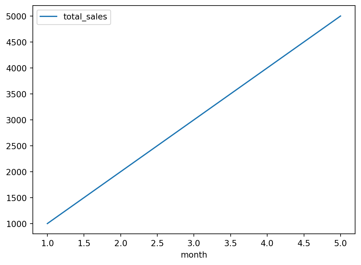

Integrating Polars with Other Data Science Tools and Libraries

Polars can be integrated with various data science tools and libraries to create a comprehensive data analysis pipeline.

Example: Using Polars with Matplotlib for Visualization

import matplotlib.pyplot as plt
# Use the previous monthly_sales DataFrame
# converted to pandas

# Plotting with Matplotlib
plt.plot(monthly_sales["month"], monthly_sales["total_sales"])
plt.title("Monthly Sales Trend")
plt.xlabel("Month")
plt.ylabel("Total Sales")
plt.show()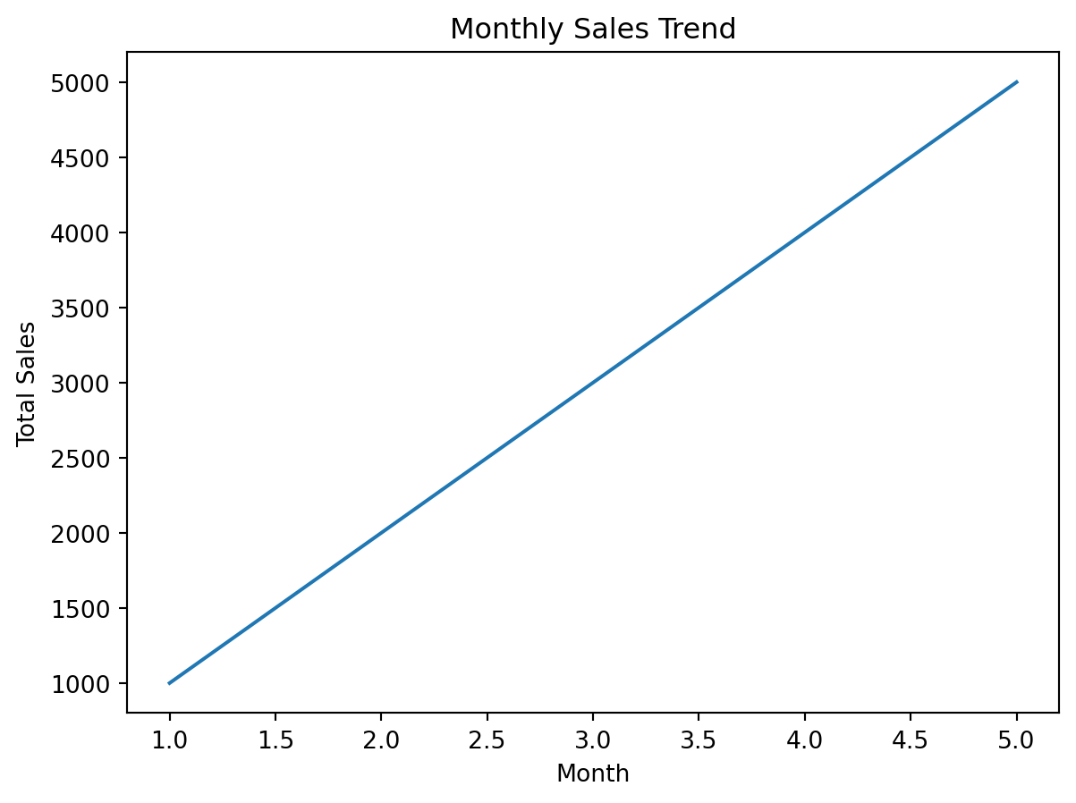

Performance Benchmarks: Polars vs. Other Libraries

Polars is known for its high performance, especially when dealing with large datasets. Let’s compare the performance of Polars with pandas, another popular data manipulation library.

Benchmarking Setup

import time
import pandas as pd
import numpy as np
# Generate a large random dataset
large_dataset = pd.DataFrame({
    "A": np.random.rand(100000000),
    "B": np.random.rand(100000000),
})
# Convert the pandas DataFrame to a Polars DataFrame
large_dataset_pl = pl.from_pandas(large_dataset)

Performance Comparison

# Pandas operation
start_time = time.time()
large_dataset["C"] = large_dataset["A"] + large_dataset["B"]
pandas_duration = time.time() - start_time
# Polars operation
start_time = time.time()
large_dataset_pl = large_dataset_pl.with_columns((pl.col("A") + pl.col("B")).alias("C"))
polars_duration = time.time() - start_time
print(f"Pandas duration: {pandas_duration}")
print(f"Polars duration: {polars_duration}")

Pandas duration: 0.13732385635375977
Polars duration: 0.08789610862731934

Tips and Tricks for Common Data Science Tasks Using Polars

Polars is not only fast but also versatile. Here are some tips and tricks for common data science tasks.

Efficient Filtering

Use Boolean expressions to filter data efficiently.

# Filter rows where sales are greater than 1000
high_sales_df = sales_df.filter(pl.col("sales_amount") > 1000)

Use Lazy Evaluation for Complex Workflows

For complex data transformations, consider using Polars’ lazy evaluation to optimize performance.

lazy_frame = sales_df.lazy()
# Define a complex transformation
lazy_result = (lazy_frame
               .with_columns(pl.col("sales_amount").cumsum().alias("cumulative_sales"))
               .filter(pl.col("cumulative_sales") < 1000000))
# Collect the result
result_df = lazy_result.collect()

Data Importing and Exporting

Finally we will explore how to import and export data using Polars, handle different data types, and manage missing values.

Reading Data from Various Sources

Polars provides a variety of functions to read data from common file formats such as CSV, JSON, Parquet, and others. Below are examples of how to read data from these sources.

Reading CSV Files

To read a CSV file, you can use the read_csv function. It allows you to specify various parameters such as file path, delimiter, and whether to infer the schema or provide it explicitly.

import polars as pl
# Read a CSV file with inferred schema
df = pl.read_csv('data.csv')
# Read a CSV file with a specified schema
schema = {'column1': pl.Int32, 'column2': pl.Float64, 'column3': pl.Utf8}
df_with_schema = pl.read_csv('data.csv', schema=schema)

Reading JSON Files

JSON files can be read using the read_json function. Polars can handle both line-delimited and nested JSON files.

# Read a line-delimited JSON file
df_json = pl.read_json('data.ldjson')
# Read a nested JSON file
df_nested_json = pl.read_json('nested_data.json')

Reading Parquet Files

Parquet is a columnar storage file format optimized for use with DataFrame libraries. Polars can read Parquet files using the read_parquet function.

# Read a Parquet file
df_parquet = pl.read_parquet('data.parquet')

Writing Data to Different File Formats

Polars also supports writing DataFrames to various file formats. Here are some examples:

Writing to CSV

To write a DataFrame to a CSV file, use the write_csv method.

# Write DataFrame to CSV
df.write_csv('output.csv')

Writing to JSON

You can write a DataFrame to a JSON file using the write_json method.

# Write DataFrame to JSON
df.write_json('output.json')

Writing to Parquet

To write a DataFrame to a Parquet file, use the write_parquet method.

# Write DataFrame to Parquet
df.write_parquet('output.parquet')

Conclusion

Polars offers a powerful and efficient way to handle and analyze data. By leveraging its performance and integrating it with other tools, you can streamline your data analysis workflows and gain valuable insights from your data.

Additional Resources

Polars User Guide: https://pola-rs.github.io/polars-book/user-guide/
Polars API Reference: https://pola-rs.github.io/polars/py-polars/html/reference/api.html
Rust Programming Language: https://www.rust-lang.org/

Glossary of Terms

DataFrame: A two-dimensional, size-mutable, potentially heterogeneous tabular data structure with labeled axes (rows and columns).
Series: A one-dimensional labeled array capable of holding any data type.
Lazy Evaluation: A programming paradigm where the evaluation of expressions is delayed until their values are needed.
Execution Plan: A representation of the sequence of operations to be performed on a DataFrame.
Parallel Execution: The process of executing multiple operations simultaneously across different CPU cores.

Troubleshooting Common Issues with Polars

Memory Errors: If you encounter memory errors, try reducing the number of threads or optimizing your data types and filters to reduce memory usage.
Performance Bottlenecks: Use profiling tools to identify slow parts of your code and consider rewriting them using Polars’ built-in functions or reordering operations to improve efficiency.